
How to Make a Table in Google Sheets: In-depth Tutorial

Google Sheets is an effective tool for creating and designing data and performing data visualizations. It offers a wide range of functionalities, and building and designing tables is just one of the many things you can execute.
The article is for beginners who just got started with Google Sheets Table. Let’s find out how to make a table in Google Sheets so that you can keep your data organized and easy to read.
Additionally, improve Google Spreadsheet table visuals and functionalities to make them more efficient.
How to create a Google Spreadsheet Table?
The fundamental concept of a table is common, although the specifics may differ depending on the spreadsheet software. In the case of Excel tables, you might not have access to all the built-in features of Google Sheets tables.
Nonetheless, it’s important to note that the functionality exists just operates distinctly. Let’s start with creating a simple table in Google Sheets.
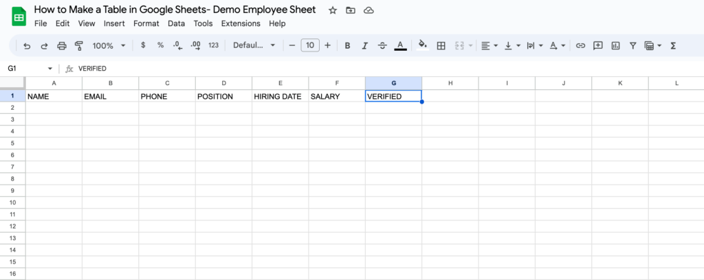
- Go to Google Sheets and add a column header
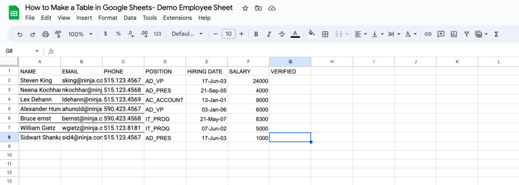
- Add your table row data
That’s how you can create a simple table in Google Sheets. Now let’s explore how to enhance the table’s appearance by applying formatting options. Additionally, we will learn how to add functionality such as filtering, collapsing, and making the table functional.
Format Google Sheet tables
Google Sheets has numerous features to make your table as beautiful as you want. When making a Google sheet table, you may want to make a table applying alternating row colors, a filtered table, or even a collapsible or searchable table as your requirements.
Let’s start with making a Google Sheet table applying alternating row colors.
Customize row colors
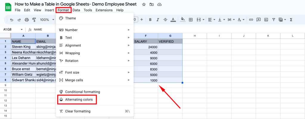
Select the range of cells containing your table, including the headers.
Go to Format > Alternating colors.
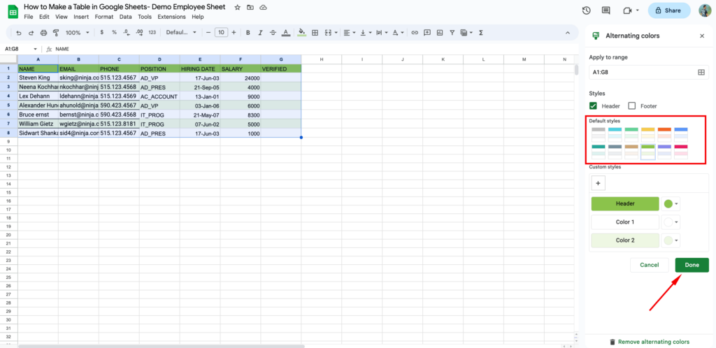
Google Sheets automatically recognizes the headers, marking the Header checkbox. If it didn’t, check the box yourself.
You can choose one of Google Sheets’ default styles or create a custom one by manually selecting the color for the header and the alternating colors for the rows. Once you’re happy with the appearance of your table, click Done.
To remove the alternating colors, click the button Remove alternating colors from the downright corner of the page. Let’s move on to the section on how to create a collapsible table in Google Sheets.
Collapsible Table in Google Sheets
When you have a large table hiding data can be error-prone. In that case, a collapsible table can be a lifesaver. You can easily organize the data in an improved way.
Rather than hiding them, you can group rows or columns to create collapsible sections.
To group table rows
- Select all rows except the headers. Or the rows you want to collapse.
- Right-click in the row number area, choose View more row actions and select Group rows.
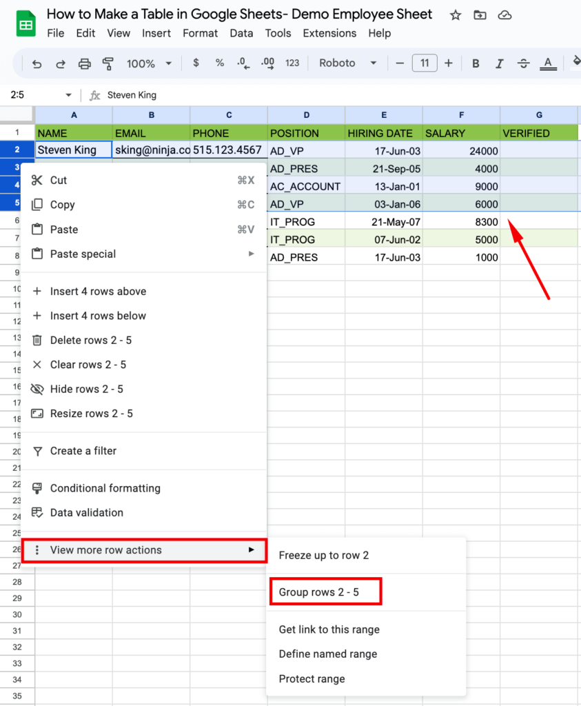
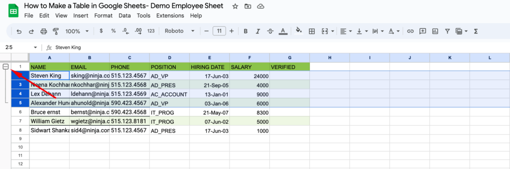
- Click the minus symbol in the top-left corner to collapse the rows.
- To expand the table, click the plus symbol in the top-left corner.
To group table columns
- Select the desired columns to collapse.
- Right-click in the column letters area, select View more column actions, and choose Group columns.
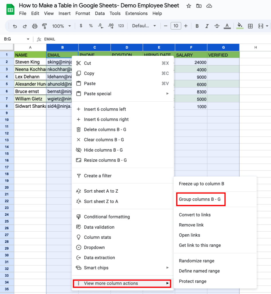
- Click the minus symbol above the first grouped column to collapse the columns.
- To expand the columns, click the plus symbol provided.
Following these steps, you can easily make your table collapsible in Google Sheets, enhancing its organization and readability. Now, let’s see how you can create a filtered table in Google Sheets.
Create a filtered table in Google Sheets
It’s worth noting that in Google Sheets, only one filtered table is allowed per sheet. If you need to use multiple filtered tables in a single file, ensure that each table is placed on a separate sheet or tab. To add filters to each column for easy data filtering and sorting, follow these steps:
- Select any header in your table. Go to Data from the admin bar. Now click on Create a filter.
- The filter icon will now appear to the right of each header. Click the filter icon in any column to access sorting and filtering options.
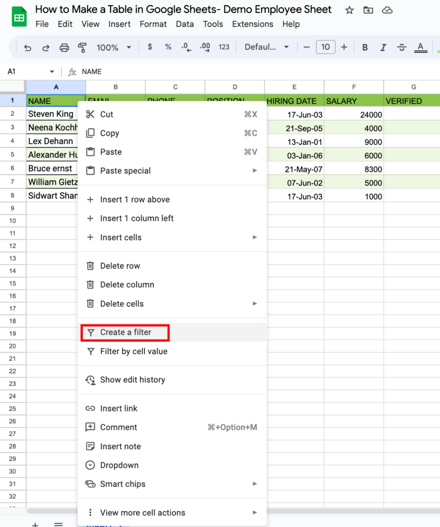
By following these steps, you can efficiently filter and sort your data in Google Sheets using the available column filters.
A functional table in Google Sheets
Using named ranges in Google Sheets can significantly save time when referring to data in tables or formulas. You can name the entire range or individual columns, allowing easy data manipulation and referencing.
Here are the steps to name your whole table and specific columns, along with examples of how to use named ranges within Google Sheets functions:
Step 01: Select the range of cells containing your table and go to Data > Named ranges. Enter the desired name for your table and click Done.
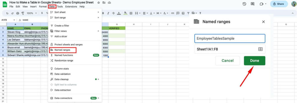
The named table will appear in the Named Ranges sidebar.
Step 02: To name a column, select it and click Add a range.
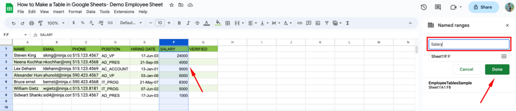
Once the column has a name, you can reference it from other cells, such as finding the total sum of purchases.
Step 03: In an empty cell, type the SUM function. After the parenthesis, start typing the exact name of the column, and select it from the suggestion box. Close the parenthesis and press Enter. You now have the sum of all purchases using the named range.
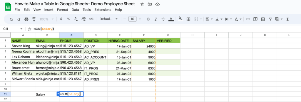
By following these steps, you can efficiently name your tables and columns, simplifying data referencing and manipulation in Google Sheets.
How to create a dropdown list in the Google Sheets table
To create a drop-down list in Google Sheets, follow these simple steps:
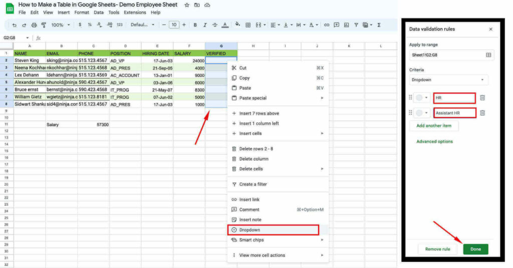
- Right-click on a cell in your Google Sheets.
- From the options that appear, select Dropdown.
- A sidebar will open on the right side of the window. In the sidebar, you can add the options that will appear in the drop-down list.
- For each option, provide a name, select a color if desired, and click Add Another Item to add more options to the list.
Embed Google Sheet tables on your website
The above section was about making a table in Google Sheets. But if you are a website owner, you need options to embed this table on it. This additional section is for those who want a table builder that enables them to embed their tables on the website.
Here, we introduce Ninja Tables, the best Google Sheet integration table to embed your tables on your web pages or posts. It comes with 100+ customization options and a lot of other exclusive features.
The best thing is the responsiveness of your table. Ninja Tables make your tables optimized for your mobile table UI. As for SEO schema, all your mobile tables will be SEO-friendly when you make your tables with Ninja Tables.
| NAME | PHONE | POSITION | HIRING DATE | SALARY | |
|---|---|---|---|---|---|
| Steven King | [email protected] | 515.123.4567 | AD_VP | 17-Jun-03 | 24000 |
| Neena Kochhar | [email protected] | 515.123.4568 | AD_PRES | 21-Sep-05 | 4000 |
| Lex Dehann | [email protected] | 515.123.4569 | AC_ACCOUNT | 13-Jan-01 | 9000 |
| Alexander Hunold | [email protected] | 590.423.4567 | AD_VP | 03-Jan-06 | 6000 |
| Bruce ernst | [email protected] | 590.423.4568 | IT_PROG | 21-May-07 | 8300 |
| William Gietz | [email protected] | 515.123.8181 | IT_PROG | 07-Jun-02 | 5000 |
| Sidwart Shankar | [email protected] | 515.123.4567 | AD_PRES | 17-Jun-03 | 1000 |
| NAME | PHONE | POSITION | HIRING DATE | SALARY | |
| Steven King | [email protected] | 515.123.4567 | AD_VP | 17-Jun-03 | 24000 |
| Neena Kochhar | [email protected] | 515.123.4568 | AD_PRES | 21-Sep-05 | 4000 |
| Lex Dehann | [email protected] | 515.123.4569 | AC_ACCOUNT | 13-Jan-01 | 9000 |
| Alexander Hunold | [email protected] | 590.423.4567 | AD_VP | 03-Jan-06 | 6000 |
| Bruce ernst | [email protected] | 590.423.4568 | IT_PROG | 21-May-07 | 8300 |
| William Gietz | [email protected] | 515.123.8181 | IT_PROG | 07-Jun-02 | 5000 |
| Sidwart Shankar | [email protected] | 515.123.4567 | AD_PRES | 17-Jun-03 | 1000 |
Get table templates for free
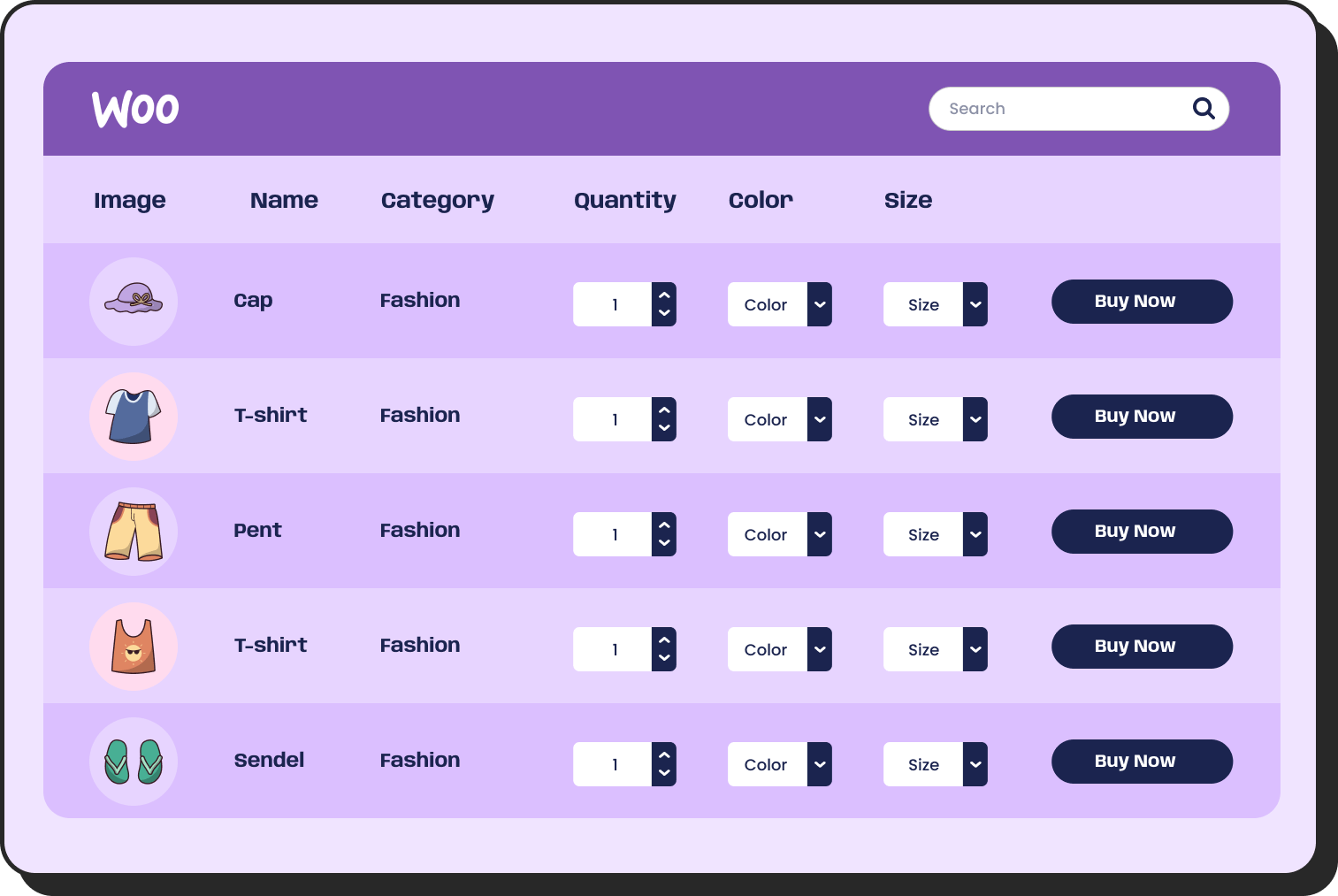
WooCommerce
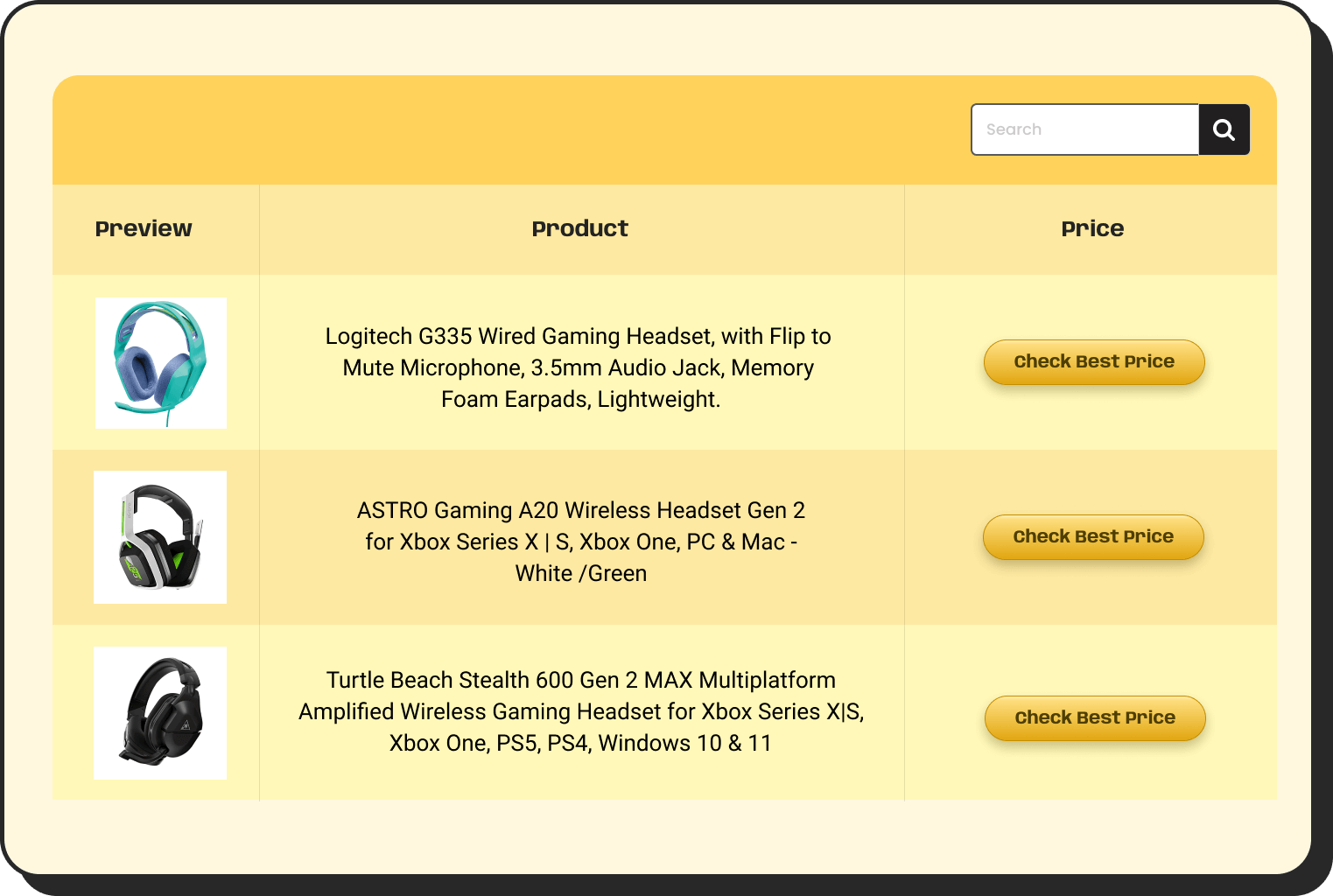
Amazon Products
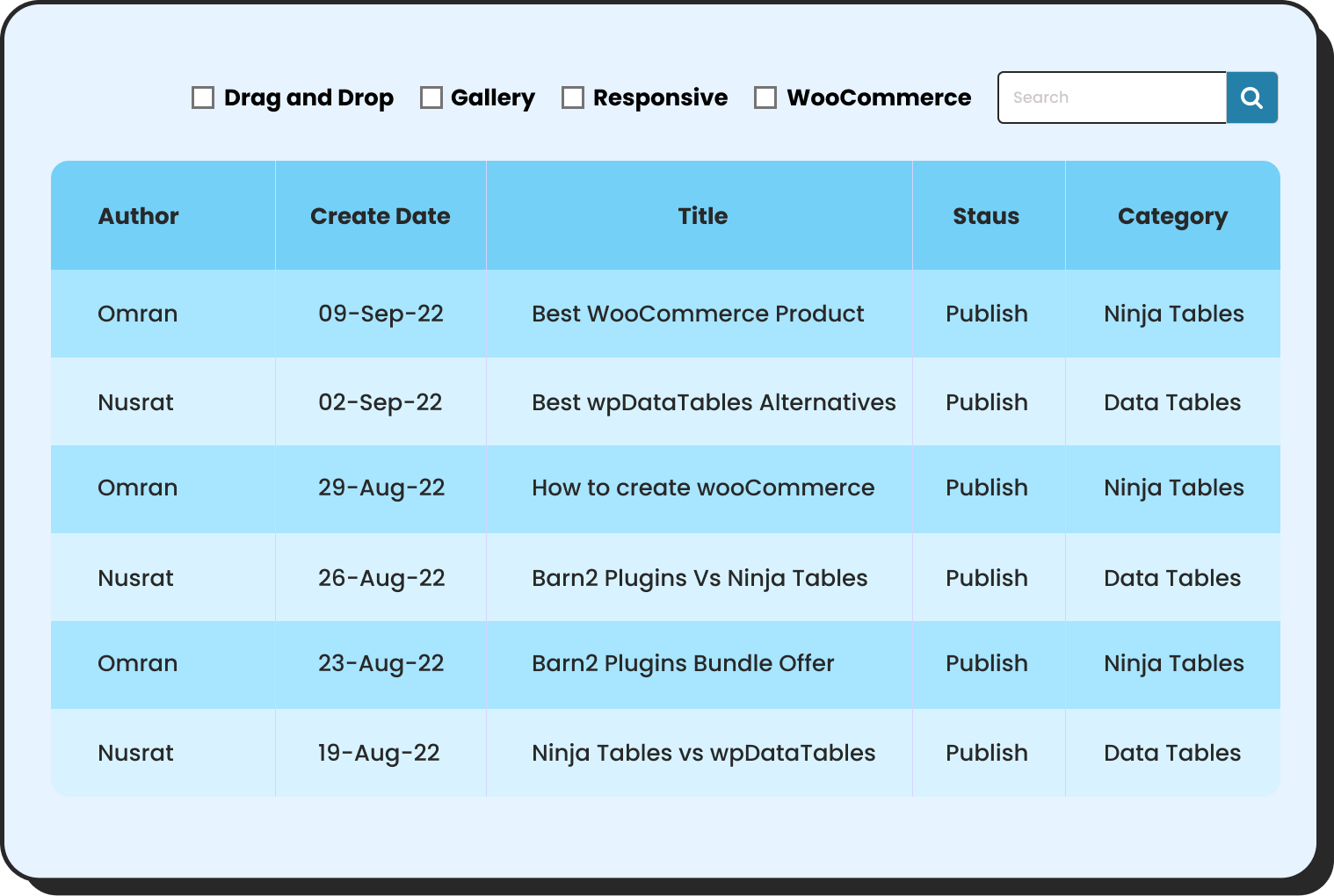
WP Posts
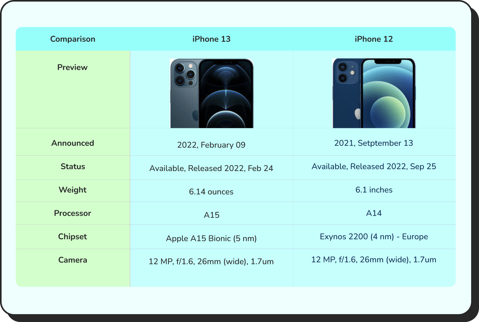
Products Comparison
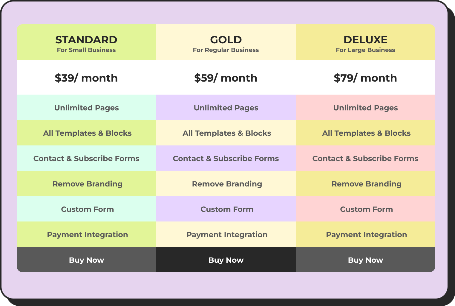
Pricing Table
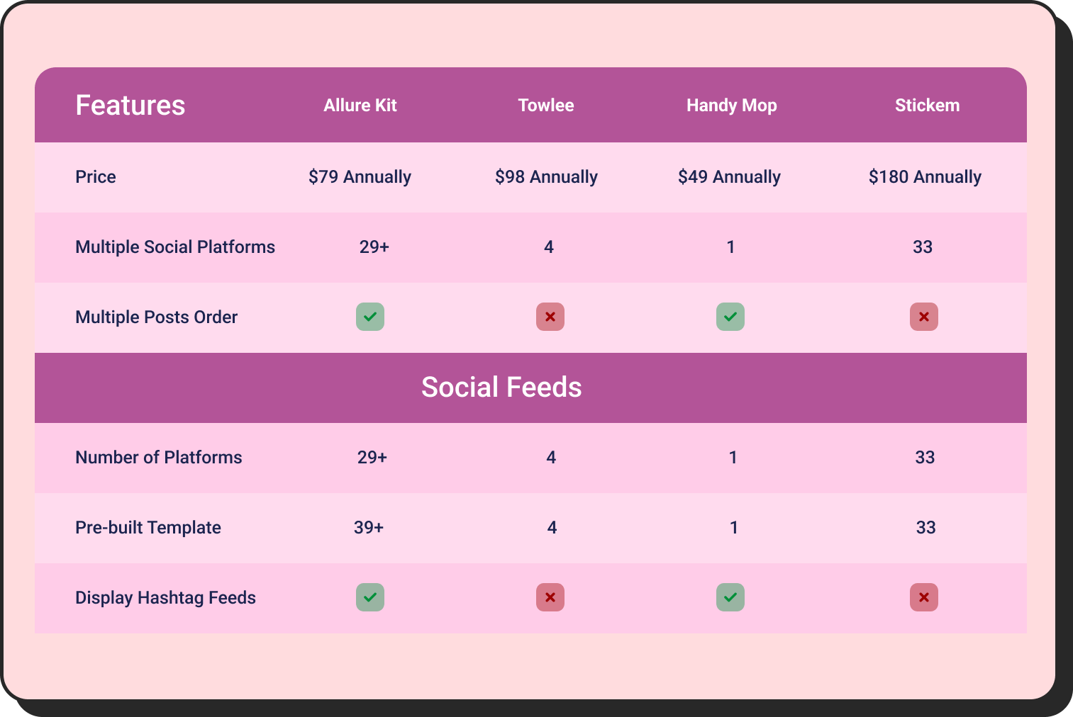
Features Comparison
Conclusion
Google Sheets offers a wide array of features that allow you to easily customize your tables according to your preferences. Additionally, you can further enhance your tables by incorporating more advanced functionalities.
By now, you are well-versed in creating basic tables effortlessly within Google Sheets. Furthermore, you have acquired techniques to improve their visual appeal through the use of distinct headers and alternating row colors.
To take your tabular data visualization to the next level, consider utilizing Ninja Tables, which seamlessly integrates with Google Sheets and enables you to showcase all your tables on your websites.
Ninja Tables– Easiest Table Plugin in WordPress
Explore our blogs on Google Sheets integration, table plugins, and tutorials for further insights. Stay updated with our social media channels for valuable tips, tricks, and updates to make your website truly amazing.


Add your first comment to this post